as I learned from the awesome book1
Jump to
Derivation of SIMPLE scheme for 1D uniform grid
A steady momentum equation may be wrote as follows.
\begin{equation}
\nabla . (\rho \overrightarrow u \overrightarrow u) = -\nabla p +  \nabla . (\mu\nabla\overline u)
\end{equation}
If it is one dimensional, the momentum and continuity equations are as follows (2) and (3):
\begin{equation}
\frac{\partial (\rho u u)}{\partial x} = - \frac{\partial p}{\partial x} + \frac{\partial}{\partial x} (\mu \frac{\partial u}{\partial x})
\end{equation}
\begin{equation}
\frac{\partial (\rho u)}{\partial x} = 0
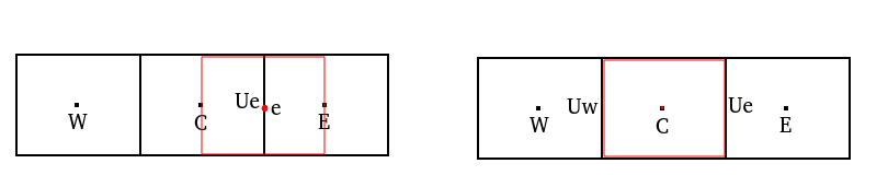
\end{equation}Representing pressure and velocity on the cell centre may lead to so called checker board problem. The solution is to adopt a staggered grid where pressures are specified at the cell centre and velocities are specified on the cell faces. The control volume for momentum and continuity equations will be different. For the momentum equation, the control volume with face as the centre will be considered while for the continuity equation, control volume will be the cell(with centre point as cell centre). Please see the figure below:
Integrating the LHS of continuity equation over the control volume,
\begin{split}
\intop_{w}^{e} \frac{\partial (\rho u)}{\partial x} \partial V &=\intop_{w}^{e} (\rho u) . ds \\&= \intop_{w}^{e}  (\rho u) \delta y \\
& \approx  \sum (\rho u)\delta y\\
& = (\rho u)_e\delta y_e - (\rho u)_w\delta y_w\\
&= m_e - m_w.
\end{split}
Considering the direction outward of the control volume negative, the continuity equation for the above referred control volume is written as :
\begin{equation}
m_{e}+ m_{w} =0 \text{  or } \sum m_{f} =0
\end{equation}
Integrating the momentum equation, (Note that cell centre is denoted by small caps in momentum control volume)
\intop_{V_{c}} \frac{\partial(\rho u u )}{\partial x} dV = \intop_{V_{c}} \frac{\partial}{\partial x}(\mu\frac{\partial u}{\partial x})dV - \intop_{V_{c}} \frac{\partial p}{\partial x}dVapplying Gauss divergence theorem except for the last term,
\intop_{\partial V_{c}} (\rho u u )dy = \intop_{\partial V_{c}}\mu \frac{\partial u}{\partial x} dy - \intop_{V_{c}} \frac{\partial p}{\partial x}dV\rho_{e}u_{e}\Delta y_{e} u_{e} - \rho_{w}u_{w}\Delta y_{w} u_{w} = (\mu \frac{\partial u}{\partial x} \Delta y)_{e} - (\mu \frac{\partial u}{\partial x} \Delta y)_{w}- \intop_{V_{c}} \frac{\partial p}{\partial x}dV[m_{e} u_{e} - m_{w} u_{w}] -[ (\mu \frac{\partial u}{\partial x} \Delta y)_{e} - (\mu \frac{\partial u}{\partial x} \Delta y)_{w}] = -\intop_{V_{c}} \frac{\partial p}{\partial x}dVTerms in the first square bracket refers to convection and second, diffusion. Both convection and diffusion terms can be written in terms of variables defined in the centre of cell under consideration and its neighbours, giving the following algebraic equation:
\begin{equation}
a_{e}u_{e} + \sum_{f} a_{f}u_{f} = b_{e} - V_{e}(\frac{\partial p}{\partial x})_{e}
\end{equation}
similarly the continuity equation can be written as: (Here small caps, because face)
\begin{equation}
\sum_{f} m_{f} = 0
\end{equation}
Derivation of pressure correction equation
Equation 5 and 6 are to be solved. Since there is no pressure term in equation 6, it is manipulated to include pressure term.
Solve the momentum equation (5) to get new values of velocity by using the initialised values for pressure p^{i}. The new values of velocity won’t be satisfying the continuity equation.
\begin{equation}
a_{e}u_{e}^{*} + \sum_{f} a_{f}u_{f}^{*} = b_{e} - V_{e}(\frac{\partial p^{i}}{\partial x})_{e}
\end{equation}
Derivation of pressure correction equation: Correction for velocity, pressure and mass are denoted as
u = u^{*} +u'\\
p = p^{*} +p'\\
m_{f} = m_{f}^{*} +m_{f}'
so the continuity equation (6) becomes
\begin{equation}
m_{e}' + m_{w}'= - (m_{e}^{*} +m_{w}^{*})
\end{equation}
where m’ is
\begin{equation}
m' = \rho .u'.\delta y
\end{equation}
to derive expression for u’, write equation (5) as
\begin{equation}
u_{e} + H_{e}(u_{e}) = B_{e} - D_{e}(\frac{\partial p}{\partial x})_{e}
\end{equation}
where,
H_{e}(u_{e}) =\sum_{f} \frac{a_{f}}{a_{e}}u_{f} \text{ , } B_{e}= \frac{b_{e}}{a_{e}} \text{ and } D_{e}= \frac{V_{e}}{a_{e}}Now for the velocities computed after solving (5),
\begin{equation}
u_{e}^{*} + H_{e}(u^{*}) = B_{e} - D_{e}(\frac{\partial p}{\partial x})_{e}
\end{equation}
Subtracting (11) from (10) gives the correction velocity
\begin{equation}
u_{e}' + \underline {H_{e}(u')} =  - D_{e}(\frac{\partial p'}{\partial x})_{e}
\end{equation}
Similarly, equation for w face can also be written.
\begin{equation}
u_{w}' + \underline {H_{w}(u')} =  - D_{w}(\frac{\partial p'}{\partial x})_{w}
\end{equation}
Since we got the expression for u’, equation (8) can be written using equations (9) as
\rho_{e} .u'_{e}.\delta y_{e} + -\rho_{w} .u'_{w}.\delta y_{w} = - (m_{e}^{*} +m_{w}^{*})Now, substituting for velocity corrections using (12) and (13),
\rho_{e} [-\underline {H_{e}(u')} - D_{e}(\frac{\partial p'}{\partial x})_{e} ]\delta y_{e} -\rho_{w} [ -\underline {H_{w}(u')} - D_{w}(\frac{\partial p'}{\partial x})_{w} ]\delta y_{w} = - (m_{e}^{*} +m_{w}^{*})now, approximating correction in gradient of pressure by considering linear variation,
-\rho_{e} D_{e}(\frac{ \delta y_{e}}{\delta x_{e}}) (p'_{E} - p'_{C}) +\rho_{w} D_{w}(\frac{ \delta y_{w}}{\delta x_{w}}) (p'_{C} - p'_{W})= - (m_{e}^{*} +m_{w}^{*}) + \rho_{e} \underline {H_{e}(u')}\delta y_{e} \\+\rho_{w} \underline {H_{w}(u')}\delta y_{w}this can be written as
\begin{equation}
a_{C}^{p'}p'_{C} + a_{E}^{p'}p'_{E} +a_{W}^{p'} p'_{W} = b_{C}^{p'}
\end{equation}
where,
a_{E}^{p'} = -\rho_{e} D_{e}(\frac{ \delta y_{e}}{\delta x_{e}})\\
a_{W}^{p'} = -\rho_{w} D_{w}(\frac{ \delta y_{w}}{\delta x_{w}})\\
a_{C}^{p'} =-(a_{E}^{p'} + a_{W}^{p'} )\\
b_{C}^{p'} =  - (m_{e}^{*} +m_{w}^{*}) + \rho_{e} \underline {H_{e}(u')}\delta y_{e} +\rho_{w} \underline {H_{w}(u')}\delta y_{w}
The SIMPLE Procedure
Step 1: Solve the momentum equation
Solve the momentum equation (5) to get new values of velocity by using the initialised values for pressure p^{i}. The new values of velocity won’t be satisfying the continuity equation.
Step 2: solve the pressure correction equation
Solve the pressure correction equation (14) to get the correction pressures.
Step3 : Calculate the velocity correction
Calculate the velocity correction from the pressure correction as
u'_{f} = - D_{f}(\frac{\partial p'}{\partial x})_{f}This is according to equation (12) or (13) where in the underlined term is neglected.
Step4 : Correct pressure and velocity
Calculate the corrected pressure and velocity field by
u^{**} = u^{*} +u'\\p^{**} = p^{*} +p'Step 5: Repeat from step 1
Set the computed pressure and velocity as new values. Go to step 1 and repeat until convergence.
SIMPLE Procedure for colocated unstructured grid
Rhie-Chow Interpolation
Employed in a colocated formulation to implicitly represent staggered formulation.
The main idea of Rhie-Chow interpolation is to write the face velocity as sum of interpolated velocity and a correction term. The correction term is proportional to the difference between two estimates of pressure gradient at the face 2.
u_{f} = \overline{u_{f}}+ \text{correction}Equation (10) shows the momentum equation for the staggered CV in which velocity is defined at the centre and pressure at the faces. If the same is applied to a colocated control volumes, with centres C and F, which are neighbours, will be
u_{C} + H_{C}(u) = B_{C} - D_{C}(\frac{\partial p}{\partial x})_{C}\\
u_{F} + H_{F}(u) = B_{F} - D_{F}(\frac{\partial p}{\partial x})_{F}
momentum equation for a control volume with intermediate face f as centre, in a similar fashion, with coefficients linearly interpolated from coefficients of momentum equations on the neighbouring cells would be :
\begin{equation}
u_{f} + \overline H_{f}(u) = \overline B_{f} - \overline D_{f}(\frac{\partial p}{\partial x})_{f}
\end{equation}
Here, the linear interpolation is carried out in the following way.
\overline \square = g_{C} \square_{C} + (1-g_{C})\square_{F}\overline H_{f} is evaluated as :
\begin{equation}
\begin{split}

\overline H_{f}(u) &=  g_{C}H_{C}(u)+(1-g_{C}) H_{F}(u)\\
&= g_{C}( -u_{C} +  B_{C} - D_{C}(\frac{\partial p}{\partial x})_{C} )+ (1-g_{C}) (-u_{F} +  B_{F} - D_{F}(\frac{\partial p}{\partial x})_{F})\\
&= -\overline u_{f} + \overline  B_{f} -\overline  {D_{f}(\frac{\partial p}{\partial x})}_{f} \\
& \approx   -\overline u_{f} + \overline  B_{f} -\overline  D_{f}\overline  {(\frac{\partial p}{\partial x})}_{f}


\end{split}
\end{equation}
with second order accuracy in approximating the RHS. We can substitute (16) in (15) to get
\begin{equation}
u_{f}  = \overline u_{f}  - \overline D_{f} ( \nabla p_{f}  -  \overline {\nabla p}_{f}   )
\end{equation}
This is called the Rhie-Chaw interpolation. In vector form,
\begin{equation}
\bold {v_{f}}  = \bold{ \overline v_{f}}  -\bold { \overline D_{f}} ( \nabla p_{f}  -  \overline {\nabla p}_{f}   )
\end{equation}
where \nabla p_{f} is obtained by modifying \overline {\nabla p_{f}} to incorporate actual gradient value in CF direction using values at C and F. That is done at the stage of gradient computation.
\nabla p_{f} = \overline {\nabla p}_{f} + (\frac {P_{F}-P_{C}}{d_{CF}} - \overline{\nabla p_{f}}.\bold{e}_{CF})\bold{e}_{CF}
Colocated pressure correction equation.
The general momentum equation can be discretised to be in the following form.
\begin{equation}
a_{C}\bold v_{C} + \sum_{F} a_{F}v_{F} = \bold b_{C}
\end{equation}
\bold b_{C} includes al the explicit terms. Non-orthogonal correction term \bold T_{f}, difference between a HR flux and upwind flux if the HR scheme is implemented via defered correction approach and \frac {1-\lambda}{\lambda} a_{C} V_{C} if relaxation is applied[pp 590].
In order to derive the pressure correction equation, the gradient term of pressure should be taken out of \bold b_{C}. Then renaming the reduced \bold b_{C} as \bold b_{C} itself,
a_{C}\bold v_{C} + \sum_{F} a_{F}v_{F} = \bold b_{C} - (\nabla p)_{C} V_{C}
Dividing the equation with a_{C},
\begin{equation}
\bold v_{C} + \bold H_{C}(\bold v) = \bold B_{C} - \bold D_{C} (\nabla p)_{C}
\end{equation}
where,
H_{C}(\bold v) =\sum_{F} \frac{a_{F}}{a_{C}}\bold v_{F} \text{ , } \bold B_{C}= \frac{\bold b_{C}}{a_{C}} \text{ and } \bold D_{C}= \frac{V_{C}}{a_{C}}Step 1 : First, solve the momentum equation with current values for velocity and previous values for pressure
\begin{equation}
\bold v_{C}^{*} + \bold H_{C}(\bold v^{*}) = \bold B_{C} - \bold D_{C} (\nabla p^{n})_{C}
\end{equation}
Defining the corrections,
\bold v = \bold v^{*} +\bold v'\\
p = p^{n} +p'\\
m_{f} = m_{f}^{*} +m_{f}'
Continuity is written as
\begin{equation}
\sum_{f} m_{f}' = - \sum_{f} m_{f}^{*} \text {  } , \text {  }where \text {  }m_{f}^{*} = \rho_{f}\bold v^{*}_{f}.\bold S_{f}
\end{equation}
The face velocity \bold v^{*}_{f} is computed using current velocities (\bold v^{*})with Rhie-Chow interpoation equation (18) as
\begin{equation}
\bold {v_{f}^{*}}  = \bold{ \overline v_{f}^{*}}  -\bold { \overline D_{f}} ( \nabla p_{f}^{n}  -  \overline {\nabla p}_{f}^{n}   )
\end{equation}
subtracting (23) from (18) gives the expression for velocity corrections.
\begin{equation}
\bold v_{f}'  = \overline { \bold v_{f}'}  -\bold { \overline D_{f}} ( \nabla p_{f}'  -  \overline {\nabla p}_{f}'   )
\end{equation}
now that the velocity corrections are estimated, it can be substituted in the continuity equation (22)
\begin{equation}
\begin{split}
- \sum_{f} m_{f}^{*} &= \sum_{f}  \rho_{f} ( \overline { \bold v_{f}'}  -\bold { \overline D_{f}} ( \nabla p_{f}'  -  \overline {\nabla p}_{f}'   ) ).\bold S_{f} \\
&=\sum_{f}  \rho_{f} \overline { \bold v_{f}'}.\bold S_{f}    - \sum_{f}\rho_{f}\bold { \overline D_{f}}  \nabla p_{f}'.\bold S_{f}  +\sum_{f} \rho_{f} \bold { \overline D_{f}}\overline {\nabla p}_{f}' . \bold S_{f} \\
&=\sum_{f}  \rho_{f} (\overline{\bold v_{f}'}+ \bold { \overline D_{f}}\overline {\nabla p}_{f}').\bold S_{f}    - \sum_{f}\rho_{f}\bold { \overline D_{f}}  \nabla p_{f}'.\bold S_{f}   \\
&=-\sum_{f}  \rho_{f} \overline {\bold H}_{f}(\bold v').\bold S_{f}    - \sum_{f}\rho_{f}\bold { \overline D_{f}}  \nabla p_{f}'.\bold S_{f}   \\
\end{split}
\end{equation}
Here, in the last step, vector form of (12) is used. Now the last term,
\begin{equation}
\begin{split}
 (\overline {\bold D}_{f}  \nabla p_{f}').\bold S_{f} &= (\nabla p_{f}' \overline {\bold D}_{f} ^{T}).\bold S_{f}  \\
&=\nabla p_{f}' .(\overline {\bold D}_{f} ^{T}.\bold S_{f})  \\
&=\nabla p_{f}' .\bold S'_{f}  (\text{ just denoting } \overline {\bold D}_{f} ^{T}.\bold S_{f} \text{ as } \bold S'_{f})\\
&=\frac{E_{f}}{d_{CF}}(p'_{F}-p'_{C})+\nabla p_{f}' .\bold T_{f}  \text{   },\text{   }where \bold S'_{f} = \bold E_{f}+\bold T_{f}\\
&\approx \frac{E_{f}}{d_{CF}}(p'_{F}-p'_{C})\text{   },\text{   neglecting}\text{   non-orthogonal} \text{   part}
\end{split}
\end{equation}
with these above, continuity equation becomes
-\sum_{f}\rho_{f}\frac{E_{f}}{d_{CF}}(p'_{F}-p'_{C}) = - \sum_{f} m_{f}^{*} -\sum_{f} \rho_{f} \overline {\bold H}_{f}(\bold v').\bold S_{f} \begin{equation}
a_{C}^{p'}p'_{C} + \sum_{F}a_{F}^{p'}p'_{F} = b_{C}^{p'}
\end{equation}a_{F}^{p'} = - \rho_{f}\frac{E_{f}}{d_{CF}}, \text{ }
a_{C}^{p'} = -\sum_{F}a_{F}^{p'}\\
b_{C}^{p'} = - \sum_{f} m_{f}^{*} -\sum_{f} \rho_{f} \overline {\bold H}_{f}(\bold v').\bold S_{f} m_{f}^{*} is calculated with (22) and (23).
Equation (27) is solved to get the correction pressure field. Then the following steps are carried out to get the corrected velocity, mass flow rate and pressure.
\begin{equation}
\begin{split}

\bold v'_{C} = -\bold D'_{C}(\nabla p')_C\\ \bold v_{C}^{**} = \bold v_{C}^{*} +\bold v'_{C}\\m_{f}' = -\rho_{f}\bold { \overline D_{f}}  \nabla p_{f}'.\bold S_{f}\\m_{f}^{**} = m_{f}^{*} +m_{f}'\\p^{**} = p^{n} +\lambda_{p} p'

\end{split}
\end{equation}
Algorithm for SIMPLE Scheme
- First, solve the momentum equation (21) with current values for velocity and previous values for pressure.
- Calculate the current mass flow rates using (22) & (23).
- Solve pressure correction equation (27) to get the correction pressures.
- Corrected values are estimated by equation (28).
- Repeat 1-4 until convergence is attained.
Prof Alberto’s wonderful brief on simple, simplec and piso is below3:
The SIMPLE algorithm in its original form (Caretto et al, 1972, Proceedings of the Third International Conference on Numerical Methods in Fluid Mechanics, Paris) is based on obtaining a pressure correction equation in which the velocity corrections are dropped because unknown (See, for example, Ferziger and Peric book). This is quite crude, and is one of the reasons why the method is not that efficient in terms of convergence rate. The effect of neglecting these terms is absent once the solution is converged however, and the method can be used “as is” for steady problems, where under-relaxation can be used to keep the solution stable.
An unsteady version of the SIMPLE algorithm can be written, by performing two loops: the external loop in time, and an internal loop to obtain a convergence solution at a given time step. In the internal loop, under-relaxation can be used, as long as a sufficient number of iterations is ensured, in order to reach the actual solution at that given time.
SIMPLEC is a version of SIMPLE where the velocity correction is introduced. However its convergence rate is very similar to what obtained with SIMPLE, using the correct under-relaxation: URF_p = 1 – URF_u (Again, see Ferziger and Peric book).
A more refined approach is the PISO one where you
- ignore the velocity corrections in the pressure equation as in the SIMPLE algorithm at the first step
- apply the velocity correction and then perform a number of other corrector steps, originating an interative procedure to solve the pressure equation treating the velocity correction term in it in an explicit manner.
as suggested by Issa (1986, Journal of Computational Physics). The PISO algorithm is considered particularly effective for unsteady flows
Source
- Moukalled F, Mangani L, Darwish M. The finite volume method in computational fluid dynamics. Berlin, Germany:: Springer; 2016.
- Fluid Mechanics 101 Rhie & Chow Interpolation (Part 3): Deriving the Correction, Sep 24, 2021
- https://www.cfd-online.com/Forums/openfoam-solving/67629-openfoam-version-1-6-details.html