as I learned from the awesome book1 and from several posts in cfdonline
This article is an outcome of an effort to learn programming in OpenFOAM. A basic conduction solver is made for the learning purpose. It is decided to document the same for the future reference. Understanding the fvMatrix (“A” matrix of Ax = b), by knowing how the contribution of boundary conditions are added to it was the main objective. Diagonal elements of A, upper elements, lower elements and source vector are printed for verification sake.
for n^{th} entry in the face list (i.e., for n^{th} face),
- n^{th} entry in the lowerAddr() : owner of the face
- n^{th} entry in the upperAddr() : neighbour of the face
- n^{th} entry in the lower() : coefficient multiplying owner variable in the equation in neighbour element
- n^{th} entry in the upper() : coefficient multiplying neighbour variable in the equation in owner element
All the above list has length equal to the number of internal faces. List diag() which carries the coefficient of cell centre variable in the present call equation has the length of number of elements.
Jump to
Making a custom solver
Step 1. Make a folder named myThermalConductionSolver (any name is fine), create a file named myThermalConductionSolver.C (any name.C) and copy the following into it.
#include "fvCFD.H"
//************************************************************//
int main(int argc, char *argv[])
{

    #include "setRootCase.H"
    #include "createTime.H"
    #include "createMesh.H"
    #include "createFields.H"

    // * * * * * * * * * * * * * * * * * * * * * * * * * * * * * * * * * * * //
    label Nc = mesh.nCells();
    Info<<"Number of Cells =  "<<Nc<<endl;
    fvScalarMatrix TEqn
    (fvm::laplacian(DT, T) + su + fvm::Sp(sp, T));

        Info<<"Diagonal elements:"<<endl<<TEqn.diag()<<endl;
        Info<<"Upper elements:"<<endl<<TEqn.upper()<<endl;
        Info<<"Lower elements:"<<endl<<TEqn.lower()<<endl;
        Info<<"boundaryCoeffs:"<<endl<<TEqn.boundaryCoeffs()<<endl;
        Info<<"internalCoeffs:"<<endl<<TEqn.internalCoeffs()<<endl;

    Info<<"Size of boundaryField is "<<T.boundaryField().size()<<endl;
    #include "defineObjectsForWriting.H"
    // Assigning contribution from BC

    forAll(T.boundaryField(), patchI)
    {
     const fvPatch &vfp = T.boundaryField()[patchI].patch();
     forAll(vfp, faceI)
     {
         label cellI = vfp.faceCells()[faceI];
         wdiag[cellI] += TEqn.internalCoeffs()[patchI][faceI];
         wsource[cellI] += TEqn.boundaryCoeffs()[patchI][faceI];
     }
    }
    // write to file
     wdiag.write();
     wsource.write();
     wlower.write();
     wupper.write();

     solve(TEqn);

     runTime++;
     runTime.write();

     Info<< nl;
     Info<< "hai from myThermalConductionSolver\n" << endl;
     return 0;
}
Please refer 2 for a complete explanation of SuSp.
patch.faceCells() will give list of cell indices for cells next to patch faces. Hence faceCells()[faceI] give the index of cell attached to that face. Hence wdiag[cellI] += TEqn.internalCoeffs()[patchI][faceI]; will add the internal coefficient of that face to the attached cell’s diagonal entry and wsource[cellI] += TEqn.boundaryCoeffs()[patchI][faceI]; will add the boundary coefficient of that face to the attached cell’s source. Looping over all patches make sure adding the internal and boundary coefficients of all boundary faces to the respective attached cells in wdiag and wsource. This is done just to print out and it does not affect the solution. In the solver, this is automatically performed while correcting the boundary conditions. See 3 and gaussLaplacianScheme.C.
solve(TEqn) calls the solver specified in fvSolution file in the system directory.
Step 2. Create a file named createFields.H and copy the following into it.
volScalarField T
(
   IOobject
   (
      "T",
      runTime.timeName(),
      mesh,
      IOobject::MUST_READ,
      IOobject::AUTO_WRITE
   ),
   mesh
);

IOdictionary transportProperties
(
   IOobject
   (
      "transportProperties",
      runTime.constant(),
      mesh,
      IOobject::MUST_READ_IF_MODIFIED,
      IOobject::NO_WRITE
   )
);

dimensionedScalar DT
(
    "DT",
    dimLength*dimLength/dimTime,
	transportProperties
);

dimensionedScalar su
(
    "su",
    dimTemperature/dimTime,
	transportProperties
);
dimensionedScalar sp
(
    "sp",
    dimless/dimTime,
	transportProperties
);
Info << "DT: " << DT << endl;
Info << "su: " << su << endl;
Info << "sp: " << sp << endl;
Step 3: Create a file named defineObjectsForWriting.H and copy the following into it
//to write
const scalarField& diag = TEqn.diag();
IOField<scalar> wdiag
(
    IOobject
    (
        "diag",
        mesh.time().timeName(),
        mesh,
        IOobject::NO_READ
    ),
    diag
);

const scalarField& upper = TEqn.upper();
IOField<scalar> wupper
(
    IOobject
    (
        "upper",
        mesh.time().timeName(),
        mesh,
        IOobject::NO_READ
    ),
    upper
);

const scalarField& lower = TEqn.lower();
IOField<scalar> wlower
(
    IOobject
    (
        "lower",
        mesh.time().timeName(),
        mesh,
        IOobject::NO_READ
    ),
    lower
);

const scalarField& source = TEqn.source();
IOField<scalar> wsource
(
    IOobject
    (
        "source",
        mesh.time().timeName(),
        mesh,
        IOobject::NO_READ
    ),
    source
);
Step 4: Create a directory named Make and create file named files in it with following contents
myThermalConductionSolver.C
EXE = $(FOAM_USER_APPBIN)/myThermalConductionSolver
Step 5: Inside the Make directory, create a file named options in it with following contents
EXE_INC = \
    -I$(LIB_SRC)/finiteVolume/lnInclude \
    -I$(LIB_SRC)/meshTools/lnInclude

EXE_LIBS = \
    -lfiniteVolume \
    -lmeshTools
Step 6: Compile the solver by running the command wmake in the myThermalConductionSolver directory. The solver is now ready which solves the Laplace equation.
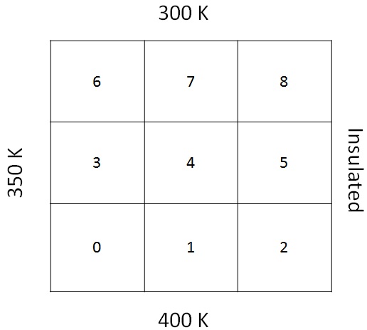
2D Diffusion example
2D steady heat conduction equation can be solved for an extremely simple geometry.
\begin{equation}
-\nabla.(\Gamma \nabla \phi) = Q_{C}
\end{equation}
Integrating within the control volume invoking the gauss divergence theorem, followed by approximating the surface integral to summation along faces,
\begin{equation}
-\sum (\Gamma \nabla \phi).S_{f} = Q_{C}V_{C}
\end{equation}
Where,
\begin  {split}
-\sum_{f} (\Gamma \nabla \phi)_{f}.S_{f} &= -\sum_{f}(\Gamma_{f} \frac{\phi_{F} -\phi_{C}}{ d_{CF}} ) S_{f}\\
 &= -\Gamma_{e} \frac{\phi_{E} -\phi_{C}}{ d_{CE}} \Delta y_{e}- \Gamma_{w} \frac{\phi_{C} -\phi_{W}}{ d_{CW}} \Delta y_{w}\\
 &-\Gamma_{n} \frac{\phi_{N} -\phi_{C}}{ d_{CN}} \Delta x_{n} -\Gamma_{s} \frac{\phi_{C} -\phi_{S}}{ d_{CS}} \Delta x_{s}\\
&= -\Gamma_{e}(\phi_{E} -\phi_{C}) \frac{\Delta y_{e}}{ d_{CE}} - \Gamma_{w} (\phi_{C} -\phi_{W})\frac{\Delta y_{w}}{ d_{CW}}\\
& -\Gamma_{n} (\phi_{N} -\phi_{C})\frac{\Delta x_{n}}{ d_{CN}} -\Gamma_{s}(\phi_{C} -\phi_{S}) \frac{\Delta x_{s}}{ d_{CS}}  \\
&= -\Gamma_{e}(\phi_{E} -\phi_{C}) \text{gDiff}_{e} - \Gamma_{w} (\phi_{C} -\phi_{W})\text{gDiff}_{w} \\
& -\Gamma_{n} (\phi_{N} -\phi_{C})\text{gDiff}_{n}-\Gamma_{s}(\phi_{C} -\phi_{S}) \text{gDiff}_{s} \\

\end{split}
Considering a neighbour cell centre F and a common face between F and C as f, the flux across the face f can be written as
-\Gamma_{f}(\phi_{F} -\phi_{C}) \text{gDiff}_{f}= FluxC_{f}\phi_{C}+FluxF_{f}\phi_{F}+ FluxV_{f}where,
FluxC_{f} =\Gamma_{f} \text{gDiff}_{f}=\Gamma_{f}\frac{\Delta y_{f}}{ d_{CF}}\\
FluxF_{f} = -\Gamma_{f}\text{gDiff}_{f}=-\Gamma_{f}\frac{\Delta y_{f}}{ d_{CF}}\\
FluxV_{f} = 0
\begin {split}
-\sum_{f} (\Gamma \nabla \phi).S_{f} &= -\Gamma_{e}(\phi_{E} -\phi_{C}) \text{gDiff}_{e} - \Gamma_{w} (\phi_{C} -\phi_{W})\text{gDiff}_{w} -\Gamma_{n} (\phi_{N} -\phi_{C})\text{gDiff}_{n}\\
& -\Gamma_{s}(\phi_{C} -\phi_{S}) \text{gDiff}_{s} \\
&= a_{C}\phi_{C} - a_{E}\phi_{E} -a_{W}\phi_{W} -a_{N}\phi_{N} -a_{S}\phi_{S}
\end{split}Where,
a_{E} = FluxF_{e} =\Gamma_{e}\text{gDiff}_{e}\\
 a_{W} = FluxF_{w} =\Gamma_{w}  \text{gDiff}_{w}\\
 a_{N} = FluxF_{n} =\Gamma_{n} \text{gDiff}_{n}\\\
 a_{S} =FluxF_{s} =\Gamma_{s} \text{gDiff}_{s}\\
\begin{split}
a_{C} &= FluxC_{e} +FluxC_{w} +FluxC_{n} +FluxC_{s} \\
&= -(a_{E} +a_{W} +a_{N} +a_{S} )
\end{split}
\begin{equation}
a_{C}\phi_{C} - a_{E}\phi_{E} -a_{W}\phi_{W} -a_{N}\phi_{N} -a_{S}\phi_{S} = b
\end{equation}where,
b = Q_{C}V_{C}-( FluxV_{e}+ FluxV_{w}+ FluxV_{n}+ FluxV_{s})Present case, Q_{C} =0.
also \Gamma = 0.1, \Delta x = \Delta y = 0.1 . Hence gDiff = 1for interior faces. For boundary faces, if temperature is specified,
-(\Gamma \nabla \phi)_{f}.S_{f} = - \Gamma_{f}\frac{\phi_{f} -\phi_{C}}{ d_{Cf}} S_{f}On a regular orthogonal grid like the present one, d_{Cf} = 0.5 d_{CF}. Hence gDiff = 2. a_{F} = \Gamma_{f} \text{gDiff}_{f} = 0.2 and FluxV_{f} =-0.2 T_{f}
a_{F} = \Gamma_{f} \text{gDiff}_{f}\\
FluxV_{f} = -\Gamma_{f} \text{gDiff}_{f}T_{f}
column 2 to 5 gives off diagonal coefficients after looping though all faces. We can see zero entries in periphery cells for a_{F} corresponding to boundary faces, since it has no neighbours. The a_{C} column is inclusive of considering internalCoeffs_ evaluated after a re-looping though boundary patches alone. A diagonal entry (coefficient of \phi_{C} of value 0.2 and source entry of 0.2 \times \T_{f} is added to all cells having temperature specified bc. For insulated(zeroGradient) boundary, \phi_{C} = \phi_{f}, hence contributions to diagonal and source entries are zeros(see element 5).
| Ele No: | a_{E} | a_{W} | a_{N} | a_{S} | FluxVe | FluxVw | FluxVn | FluxVs | a_{C} | b |
| 0 | -0.1 | 0 | -0.1 | 0 | 0 | -70 | 0 | -80 | 0.6 | 150 |
| 1 | -0.1 | -0.1 | -0.1 | 0 | 0 | 0 | 0 | -80 | 0.5 | 80 |
| 2 | 0 | -0.1 | -0.1 | 0 | 0 | 0 | 0 | -80 | 0.4 | 80 |
| 3 | -0.1 | 0 | -0.1 | -0.1 | 0 | -70 | 0 | 0 | 0.5 | 70 |
| 4 | -0.1 | -0.1 | -0.1 | -0.1 | 0 | 0 | 0 | 0 | 0.4 | 0 |
| 5 | 0 | -0.1 | -0.1 | -0.1 | 0 | 0 | 0 | 0 | 0.3 | 0 |
| 6 | -0.1 | 0 | 0 | -0.1 | 0 | -70 | -60 | 0 | 0.6 | 130 |
| 7 | -0.1 | -0.1 | 0 | -0.1 | 0 | 0 | -60 | 0 | 0.5 | 60 |
| 8 | 0 | -0.1 | 0 | -0.1 | 0 | 0 | -60 | 0 | 0.4 | 60 |
\begin  {split}
T_{0} &=  (0.1 T_{1}+0.1 T_{3}+150)/0.6\\
T_{1} &=  (0.1 T_{0}+0.1 T_{2}+0.1 T_{4}+80)/0.5\\
T_{2} &=  (0.1 T_{1}+0.1 T_{5}+80)/0.4\\
T_{3} &=  (0.1 T_{0}+0.1 T_{4}+0.1 T_{6}+70)/0.5\\
T_{4} &=  (0.1 T_{1}+0.1 T_{3}+0.1 T_{5}+0.1 T_{7}+70)/0.4\\
T_{5} &=  (0.1 T_{3}+0.1 T_{4}+0.1 T_{8})/0.3\\
T_{6} &=  (0.1 T_{3}+0.1 T_{7}+130)/0.6\\
T_{7} &=  (0.1 T_{4}+0.1 T_{6}+0.1 T_{8}+60)/0.5\\
T_{8} &=  (0.1 T_{5}+0.1 T_{7}+60)/0.4\\

\end{split}
Manual solution
This can be solved iteratively, the easiest by filling a single column 8 raw in excel file with 300. Write equations in the next column against each row. Copy and paste the column 5 or 6 times towards right to get an approximate solution.
Solution in OpenFOAM
constant/polyMesh/blockMeshDict
/*--------------------------------*- C++ -*----------------------------------*\
 | ========= | |
 | \\      / F ield | OpenFOAM: The Open Source CFD Toolbox |
 |  \\    /  O peration | Version: 2.1.1 |
 |   \\  /   A nd | Web: www.OpenFOAM.org |
 |    \\/    M anipulation |
 |
\*---------------------------------------------------------------------------*/
FoamFile
{
version 2.0;
format ascii;
class
 dictionary;
object blockMeshDict;
}
// * * * * * * * * * * * * * * * * * * * * * * * * * * * * * * * * * * * * * //
convertToMeters 1;
vertices
(
(0 0 0)
(0.3 0 0)
(0.3 0.3 0)
(0 0.3 0)
(0 0 1)
(0.3 0 1)
(0.3 0.3 1)
(0 0.3 1)
);
blocks
(
hex (0 1 2 3 4 5 6 7) (3 3 1) simpleGrading (1 1 1)
);
edges
(
);
boundary
(
left
{
type wall;
faces
(
(4 7 3 0)
);
}
right
{
type wall;
faces
(
(2 6 5 1)
);
}
top
{
type wall;
faces
(
(2 3 7 6)
);
}
bottom
{
type wall;
faces
(
(1 5 4 0)
);
}
frontAndBack
{
type empty;
faces
(
(0 3 2 1)
(4 5 6 7)
);
mergePatchPairs
(
);
// ************************************************************************* //
constant/transportProperties
/*--------------------------------*- C++ -*----------------------------------*\
 | ========= | |
 | \\      / F ield | OpenFOAM: The Open Source CFD Toolbox |
 |  \\    /  O peration | Version: 2.1.1 |
 |   \\  /   A nd | Web: www.OpenFOAM.org |
 |    \\/    M anipulation |
 |
\*---------------------------------------------------------------------------*/
FoamFile
{
version 2.0;
format ascii;
class
dictionary;
location "constant";
object transportProperties;
}
// * * * * * * * * * * * * * * * * * * * * * * * * * * * * * * * * * * * * * //
DT
DT [ 0 2 -1 0 0 0 0 ] 0.1;
su
su [ 0 0 -1 1 0 0 0 ] 0.0;
sp
sp [ 0 0 -1 0 0 0 0 ] 0.0;
// * * * * * * * * * * * * * * * * * * * * * * * * * * * * * * * * * * * * * //
system/controlDict
/*--------------------------------*- C++ -*----------------------------------*\
 | ========= | |
 | \\      / F ield | OpenFOAM: The Open Source CFD Toolbox |
 |  \\    /  O peration | Version: 2.1.1 |
 |   \\  /   A nd | Web: www.OpenFOAM.org |
 |    \\/    M anipulation |
 |
\*---------------------------------------------------------------------------*/
FoamFile
{
version 2.0;
format ascii;
class
 dictionary;
location "system";
object controlDict;
}
// * * * * * * * * * * * * * * * * * * * * * * * * * * * * * * * * * * * * *application
 myThermalConductionSolver;
startFrom
 startTime;
startTime
 0;
stopAt
 endTime;
endTime
 1;
deltaT
 1;
writeControl runTime;
writeInterval 1;
purgeWrite
 0;
writeFormat
 ascii;
writePrecision 6;
writeCompression off;
timeFormat
 general;
timePrecision 6;
runTimeModifiable true;
|
//
// ************************************************************************* //
system/fvSchemes
/*--------------------------------*- C++ -*----------------------------------*\
 | ========= | |
 | \\      / F ield | OpenFOAM: The Open Source CFD Toolbox |
 |  \\    /  O peration | Version: 2.1.1 |
 |   \\  /   A nd | Web: www.OpenFOAM.org |
 |    \\/    M anipulation |
 |
\*---------------------------------------------------------------------------*/
FoamFile
{
version 2.0;
format ascii;
class
 dictionary;
location "system";
object fvSchemes;
}
// * * * * * * * * * * * * * * * * * * * * * * * * * * * * * * * * * * * * *ddtSchemes
{
default
}
steadyState;
gradSchemes
{
default
 Gauss linear;
grad(T)
 Gauss linear;
}
divSchemes
{
default
}
none;
laplacianSchemes
{
default
 none;
laplacian(DT,T) Gauss linear uncorrected;
}
interpolationSchemes
{
default
 linear;
}
snGradSchemes
{
default
 none;
}
fluxRequired
{
default
T
 ;
}
no;
// ************************************************************************* //
system/fvSolution
/*--------------------------------*- C++ -*----------------------------------*\
 | ========= | |
 | \\      / F ield | OpenFOAM: The Open Source CFD Toolbox |
 |  \\    /  O peration | Version: 2.1.1 |
 |   \\  /   A nd | Web: www.OpenFOAM.org |
 |    \\/    M anipulation |
 |
\*---------------------------------------------------------------------------*/
FoamFile
{
version 2.0;
format ascii;
class
 dictionary;
location "system";
object fvSolution;
}
// * * * * * * * * * * * * * * * * * * * * * * * * * * * * * * * * * * * * * //
solvers
{
T
{
solver
 PBiCG;
preconditioner DILU;
tolerance
 1e-06;
relTol
 0;
}
}
SIMPLE
{
nNonOrthogonalCorrectors 0;
}
// ************************************************************************* //
0/T
/*--------------------------------*- C++ -*----------------------------------*\
 | ========= | |
 | \\      / F ield | OpenFOAM: The Open Source CFD Toolbox |
 |  \\    /  O peration | Version: 2.1.1 |
 |   \\  /   A nd | Web: www.OpenFOAM.org |
 |    \\/    M anipulation |
 |
\*---------------------------------------------------------------------------*/
FoamFile
{
version 2.0;
format ascii;
class
 volScalarField;
object T;
}
// * * * * * * * * * * * * * * * * * * * * * * * * * * * * * * * * * * * * * //
dimensions
internalField[0 0 0 1 0 0 0];
uniform 300;
boundaryField
{
left
{
type
 fixedValue;
value
 uniform 350;
}
right
{
type
 zeroGradient;
}
top
{
type
 fixedValue;
value
 uniform 300;
}
bottom
{
type
 fixedValue;
value
 uniform 400;
}
frontAndBack
{
type
empty;
// ************************************************************************* //
Run the case calling blockMesh followed by myThermalConductionSolver.
Results
1/T

dimensions
 [0 0 0 1 0 0 0];
internalField nonuniform List<scalar> 9(371.818 380.909 382.727 350 350 350 328.182 319.091
317.273);
0/diag
9(-0.6 -0.5 -0.4 -0.5 -0.4 -0.3 -0.6 -0.5 -0.4)
0/lower
12 (0.1 0.1 0.1 0.1 0.1 0.1 0.1 0.1 0.1 0.1 0.1 0.1 )
0/upper
12 (0.1 0.1 0.1 0.1 0.1 0.1 0.1 0.1 0.1 0.1 0.1 0.1 )
0/source
9(-150 -80 -80 -70 0 0 -130 -60 -60)
- Size of upper and lower is equal to the total number of internal faces. For the type of mesh considered here, it is m(n-1)+n(m-1), where m and n are number of rows and columns respectively.
- diag shows the list of coefficient multiplying the variable defined in the respective cell for each cell. Initially, the contribution of internal faces are constdered. Hence, the diag is calculated as 9(-0.2 -0.3 -0.2 -0.3 -0.4 -0.3 -0.2 -0.3 -0.2). Subsequently, the contribution from boundary faces(FluxCc: internal coefficients ) are added to become 9(-0.6 -0.5 -0.4 -0.5 -0.4 -0.3 -0.6 -0.5 -0.4) .
- internalCoeffs is like a vector of 1-d vectors. No. of 1-d vectors equal to the number of boundary patches, which is 5 here left, right, top, bottom and the frontAndBack boundary patch. Size of each 1-d vector is the number of faces in the respective boundary patch. Each entry is the coefficient multiplying the variable defined in the owner cell of the respective faces.
Symmetric/Asymmetric
- One could easily see that the matrix is symmetric but still the solver require an asymmetric matrix solver (eg. PBiCG). This is because, if fvMatrix object has both upper() and lower(), then the matrix is treated as asymmetric.
- If only one of the lower or upper triangles are defined, the matrix is assumed to be symmetric. If both are defined, it will assume the matrix is asymmetric, even if they are equal. Accessing the opposite pointer without a const modifier will convert the matrix to an asymmetric matrix. To modify the off-diagonal of a symmetric matrix, first test which pointer is active using hasUpper() and hasLower() 4
- In the code, if we avoid defining/accessing lower() (or upper())then the matrix is treated as symmetric and then we need to make changes in the fvSolution file for solver and preconditioner that suit symmetric matrix.
internalCoeffs:
5
(
3(-0.2 -0.2 -0.2)
3{0}
3(-0.2 -0.2 -0.2)
3(-0.2 -0.2 -0.2)
0()
)
- boundaryCoeffs is like internalCoeffs but the entry in each 1-d vector is the value of flux at respective faces.
boundaryCoeffs:
5
(
3(-70 -70 -70)
3{0}
3(-60 -60 -60)
3(-80 -80 -80)
0()
)
- boundaryCoeffs when added to the respective owner cells make the source vector: 9(-150 -80 -80 -70 0 0 -130 -60 -60)
Effect of adding source
su =1, sp = 0 case
- If we keep su=1 in constant/tansportProperties, the source is modified from 9(-150 -80 -80 -70 0 0 -130 -60 -60) to 9(-150.01 -80.01 -80.01 -70.01 -0.01 -0.01 -130.01 -60.01 -60.01).
- su is multiplied by volume 0.01(0.1m*0.1m*1m here) and added to the source term.
- upper, lower and diag remain same. Temp is 9(371.854 380.969 382.795 350.053 350.096 350.11 328.217 319.151 317.34);
su = 0, sp =1 case
- Only diag value before adding bc effect changes from 9(-0.2 -0.3 -0.2 -0.3 -0.4 -0.3 -0.2 -0.3 -0.2) to 9(-0.19 -0.29 -0.19 -0.29 -0.39 -0.29 -0.19 -0.29 -0.19)
- This is because sp is +ve and it is added to the fvMatrix after multiplying with volume 0.01
- upper, lower and source remain same
- T = 9(385.473 404.352 409.393 369.939 386.458 392.282 340.771 340.612 341.768);
fvm::Sp function defined in $FOAM_SRC/finiteVolume/finiteVolume/fvm/fvmSup.C is used here. Sp is defined as
template<class Type>
Foam::tmp<Foam::fvMatrix<Type> >
Foam::fvm::Sp
(
const DimensionedField<scalar, volMesh>& sp,
const GeometricField<Type, fvPatchField, volMesh>& vf
)
{
const fvMesh& mesh = vf.mesh();
tmp<fvMatrix<Type> > tfvm
(
new fvMatrix<Type>
(
vf,
dimVol*sp.dimensions()*vf.dimensions()
)
);
fvMatrix<Type>& fvm = tfvm();
fvm.diag() += mesh.V()*sp.field();
return tfvm;
}
The resulting matrix is just added in the equation.
Source
- Moukalled F, Mangani L, Darwish M. The finite volume method in computational fluid dynamics. Berlin, Germany:: Springer; 2016.
- cfd-online:fvmatrix-fvoptions-susp-automatic-implicit-explicit-source-term-treatment
- gaussLaplacianScheme(1/2): Theory and implementation in OpenFOAM
- https://openfoamwiki.net/index.php/OpenFOAM_guide/Matrices_in_OpenFOAM