Multiphase flow modelling – 2: Lagrangian particle tracking

Parameters

• Maximum number of particles: npmax
• Particle diameter: dp
• Particle density: rhop
• Fluid density: rhof
• Particles flow rate: PFR (number of particles entering per second)
• Particle inlet velocity: up_in
• Two-way coupling(Boolean): use_twoway

Define a derived data type for particle with following detail

• double x, y : position
• int i,j : mesh location
• double u,v : velocity
• double dt : Time step size
• int or boolean stop: active or not

Create an array of particles part, ptmp

Identify the current mesh location(i,j) of the particle based on particle position

This is rather easy in a structured grid compared to an unstructured one. The idea is particle would be somewhere near to the location it was at the previous time step. Hence we shall search the immediate four(in 2D) neighbours and if not found, search neighbours’ neighbours.

Algorithm

• grab the old location: iold, jold
• grab the current position: xp, yp
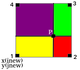
• define now location: inew, jnew
• Search to the right: do while (xp >=x(inew+1) && inew+1 <= nx); inew=inew+1;
• Search to the left: do while (xp <= x(inew) && inew-1>= 1 ); inew=inew-1;
• Either of the above search will only execute.
• Do the same for yp

Bilinear interpolation

The new location we arrive is marked in the figure below. Linearly interpolate for U & V.

U_{P} = \frac{U1*Green+U2*Purple+U3*Yellow+U4*Red}{Green+Purple+Yellow+Red}

wx1=(x0-x (i))/(x (i+1)-x (i)); wx2=1.0_WP-wx1
wy1=(y0-ym(j))/(ym(j+1)-ym(j)); wy2=1.0_WP-wy1
// Rectangular area in a matrix
    ww(1,1)=wx1*wy1
    ww(2,1)=wx2*wy1
    ww(1,2)=wx1*wy2
    ww(2,2)=wx2*wy2
 //Bilinear interpolation of U
    myu=sum(ww*U(i:i+1,j:j+1))

Particle initialisation

particles to be added nadd = PFR*dt

for 0:nadd, do the following

• nadded++, np++
• give x position that of inlet
• y position random between y(1) and y(ny)
• locate i,j using previously defined plocate algorithm
• If any particle are in wall (mask ==1), remove that particle (nadded++, np++)
• Initialise u velocity to the particle

ODE solver for a single particle: Second order Runge-Kutta

Step 1: Predictor (Forward Euler) : \phi^{n+\frac{1}{2}} = \phi^{n} + \frac{\Delta t}{2}f(\phi^{n})

Step 2: Corrector (Centered in time) : \phi^{n+1} = \phi^{n} +\Delta tf(\phi^{n+\frac{1}{2}})

Algorithm

for each particle p

Predictor – Euler prediction

• copy p to pn
• Calculate drag(dragx and dragy) by calling lpt_drag(dragx,dragy).
• p.x = pn.x +0.5*p.dt *p.u
• p.y = pn.y +0.5*p.dt *p.v
• p.u = pn.u +0.5*p.dt *(dragx+gravity_x+collision_x)
• p.v = pn.v +0.5*p.dt *(dragy+gravity_y+collision_y)

Corrector – Midpoint rule

• Recalculate drag(dragx and dragy) by calling lpt_drag(dragx,dragy).
• p.x = pn.x +p.dt *p.u
• p.y = pn.y +p.dt *p.v
• p.u = pn.u +p.dt *(dragx+gravity_x+collision_x)
• p.v = pn.v +p.dt *(dragy+gravity_y+collision_y)

call plocate to relocalize particle on mesh

Update optimal timestep size p.dt=taup

Drag Model (lpt_drag(dragx,dragy).)

Step 1: Obtain particle velocity by interpolation. Input: i,j,x,y Output: u,v

ug=get_u(p.i,p.j,p.x,p.y) and vg=get_v(p.i,p.j,p.x,p.y)

Step 2: Calculate Stokes response time

taup=dp^2/(18.0*knu)

Step 3: Calculate particle Reynolds number

Step 4: Shiller & Naumann drag correlation

taup=taup/(1.0+0.15*Rep*(0.687))

Step 5: Acceleration due to drag
accx=(ug – p.u)/taup
accy=(vg – p.v)/taup

accx, accy are dragx and dragy

two way coupling

For two-way coupling, add momentum source term calculated from particle to the u* calculation in the velocity step.

 // Increment exchange term
  if (mask(myp%i,myp%j).eq.0) then
     loading=rhop*Pi/6.0_WP*dp**3/(rhof*d**3)//ratio of particlemass tot fluid mass
     tmpU(myp%i,myp%j)=tmpU(myp%i,myp%j)-mydt*dragx*loading
     tmpV(myp%i,myp%j)=tmpV(myp%i,myp%j)-mydt*dragy*loading
  end if

// Transfer source to flow solver
  if (use_twoway) then
     do j=1,ny
        do i=2,nx
           if (maxval(mask(i-1:i,j)).eq.0) srcU(i,j)=srcU(i,j)+0.5_WP*sum(tmpU(i-1:i,j))
        end do
     end do
     do j=2,ny
        do i=1,nx
           if (maxval(mask(i,j-1:j)).eq.0) srcV(i,j)=srcV(i,j)+0.5_WP*sum(tmpV(i,j-1:j))
        end do
     end do
  end if

//In velocity_step
// Adams-Bashforth
  U=U+HU1+ABcoeff*(HU1-HU2)+srcU
  V=V+HV1+ABcoeff*(HV1-HV2)+srcV