Multiphase flow modelling – 1: Development of a basic flow solver

learned from Oliver Desjardins’ lecture (notes)

Development of a basic flow solver¹

• Incompressible flow
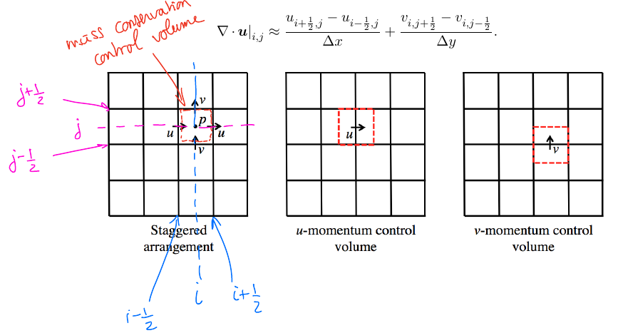
• Structured 2D staggered grid
• P-U coupling by Fractional Step Method(simplified version of Kim and Moin, 1985)

2d N-S eqn

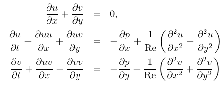
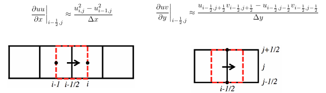
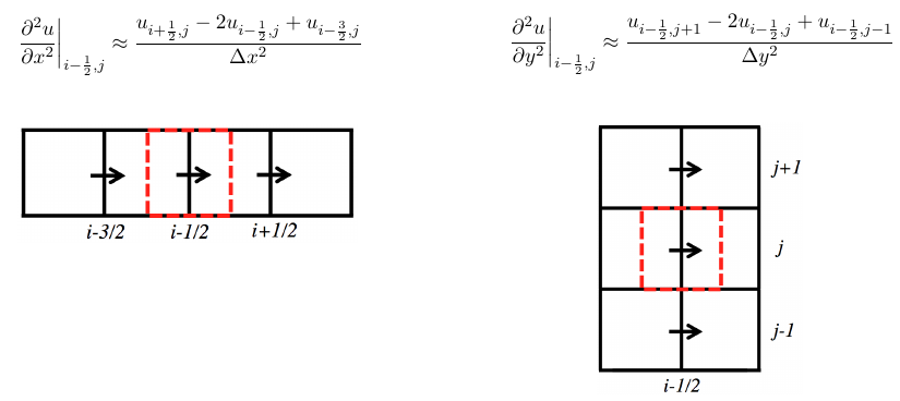
Spatial discretization

Gradient and Laplacian term of pressure by standard second order central differensing scheme.

The fractional step method

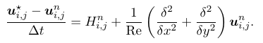
Original fractional step method by Kim and Moin (1985) uses explicit Adams–Bashforth discretization of the convective term with a Crank–Nicolson discretisation of the viscous term, and uses a projection idea to handle the pressure coupling. Here, we simplify viscous term by using first order explicit forward in time.

Step 1. The momentum equations are advanced without a pressure term

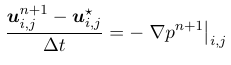
Step 2 : Projection

Effect of pressure shall be introduced to take us from intermediate velocity to velocity at next time step .

Wikipedia says: Helmholtz’s theorem, also known as the fundamental theorem of vector calculus, states that any sufficiently smooth, rapidly decaying vector field can be resolved into the sum of an irrotational (curl-free) vector field and a solinoidal (divergence-free) vector field; this is known as the Helmholtz decomposition.

Hence what we do is, get the curl-free part and subtract from intermediate velocity to arrive at solinoidal (divergence-free) part of velocity. Also see² from 11:30s onwards

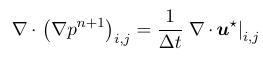
Taking divergence of the above equation and enforcing solinoid property for velocity at next time step,

Pressure laplacian

Gradient of pressure is curl free, since curl of gradient of a scalar field equals zero: ³A scalar field is single valued. That means that if you go round in a circle, or any loop, large or small, you end up at the same value that you started at. The curl of the gradient is the integral of the gradient round an infinitesimal loop which is the difference in value between the beginning of the path and the end of the path. In a scalar field there can be no difference, so the curl of the gradient is zero.

Velocity correction

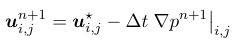
subtract curl-free part from intermediate velocity to get velocity at next time step

Algorithm

Step 1: Define parameters

• number of divisions in x and y nx,ny
• maxdt, maxCFL,maxtime,maxstep(max time step)
• relative and absolute convergence relcvg, abscvg
• Domain size Lx, Ly
• fluid property kinematic viscosity knu.

Step 2: Define mesh and solution vectors

• Mesh: x,y, centroids xm, ym, boolean mask for noting solid/fluid domain
• Solution vectors U,V,P
• Residual vectors HU1, HV1 and HU2, HV2 for storing old values
• Velocity divergence div
• 2D array of laplacian stencils plap, ulap, vlap in x and y

Step 3: Initialise

• Apply Neumann condition on masks: mask( 0,:)=mask( 1,:), mask(nx+1,:)=mask(nx,:), mask(:, 0)=mask(:, 1), mask(:,ny+1)=mask(:,ny)
• Add ghost cells to periphery
• Fill pressure laplacian vector array by value [\frac{1}{d^{2}}, \frac{-2}{d^{2}}, \frac{1}{d^{2}}]
• Apply Neumann conditions for pressure laplacian to ensure zero gradient at all sides. e.g., at left side of domain, plap(1,:,1, 0)=plap(1,:,1,0)+plap(1,:,1,-1) and plap(1,:,1,-1)=0.0. Here plap is plap(i,j,x/y,stencil(-1,0,1)) where stencil(-1,0,1) is coeff multiplying corresponding U(i) or V (i)
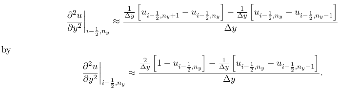
• Modify laplacian to handle wall. If (mask(i,j)==1) then plap stencil is (0,1,0). If cell is neighbor to wall , use Neumann. e.g.,for right side of current cell, if (mask(i+1,j).eq.1) then plap(i,j,1, 0)=plap(i,j,1,0)+plap(i,j,1,+1) and plap(i,j,1,+1)=0. Do for all sides of cell.
• Fill u and v laplacian vector array by value [\frac{1}{d^{2}}, \frac{-2}{d^{2}}, \frac{1}{d^{2}}]
• Apply Dirichlet bc (0 or value): u (x = 0, y) = 0 , u (x = 1, y) = 0, v (x, y = 0) = 0, v (x, y = 1) = 0.
• But these value we apply at cell centre. It should’ve been at boundary face. So correction is needed.viscous stencil at the walls need to become asymmetric for y-viscous term for u at the top and bottom wall, and for the x-viscous term for v at the left and right walls as shown below: For y-viscous term for u at the top wall (which , say moves at 1 m/s right) change

Step 4: Velocity step: find out intermediate velocity

• Since it is in an loop, first copy the residual vectors HU1, HV1 to corresponding old vectors HU2, HV2.
• Calculate residuals (sum of convective and viscous terms) in u and v momentum equation

HU1(i,j)=-conv*((U(i,j  )+U(i+1,j))*(U(i,j  )+U(i+1,j  ))-(U(i-1,j)+U(i,j  ))*(U(i-1,j)+U(i  ,j))) -conv*((U(i,j+1)+U(i  ,j))*(V(i,j+1)+V(i-1,j+1))-(U(i  ,j)+U(i,j-1))*(V(i  ,j)+V(i-1,j))) +visc*(sum(ulap(i,j,1,-1:+1)*U(i-1:i+1,j))+sum(ulap(i,j,2,-1:+1)*U(i,j-1:j+1)))

• Use Adams-Bashforth to get intermediate velocities U=U+HU1+ABcoeff(HU1-HU2) and V=V+HV1+ABcoeff(HV1-HV2)
• Apply Neumann and DIrichlet boundary conditions at domain edges

Step 5: Pressure poisson

• Enforce global mass conservation. If right is outflow, U(nx+1,j)=U(nx+1,j)+(left_mfr*left_area/right_area-right_mfr)
• Compute divergence div(i,j)=[ U(i+1,j)-U(i,j) + V(i,j+1)-V(i,j) ] /d
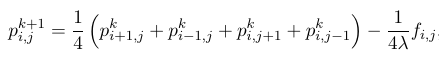
• Iterate pressure poisson eqn to get p(i,j) values. Here PCG with DIC as P is used.

Step 6: Velocity correction

• Correct U by U(i,j)=U(i,j)-dt*(P(i,j)-P(i-1,j))/d and V by V(i,j)=V(i,j)-dt*(P(i,j)-P(i,j-1))/d
• Recalculate divergence div(i,j)=(U(i+1,j)-U(i,j)+V(i,j+1)-V(i,j))/d

Step 7: Advance time

• Calculate max CFL is follows

  CFL=0.0
  for j=1:ny{
     for i=1:nx{
        CFL=max(CFL,abs(U(i,j))/d)
        CFL=max(CFL,abs(V(i,j))/d)
        CFL=max(CFL,4.0*knu/d^2)
     }
  }
  CFL=CFL*dt

• Calculate time step

dt_old=dt
dt=min(maxCFL/(CFL+epsilon(1.0_WP))*dt_old,maxdt)

• Advance time: t = t + dt

1. Multiphase flow modelling lecture by Oliver Desjardins
2. How DO Fluid Simulations Work?
3. physical meaning of curl of gradient of a scalar field equals zero