Flow of immiscible fluids can be segregated, mixed or dispersed. If you slightly tilt a water bottle, the minor oscillations you see describe a segregated flow. If you swing it moderately, a mildly violent sloshing happens at the interface causing a few droplets jump out of the interface. This could be called a mixed flow. But if you wildly shake a half emptied bottle, the air bubbles seem suspended in the water and you see a dispersed system.
The main focus of this article is on modelling of segregated flows. This post is the result of my quick reading of the doctoral thesis of Onno Ubbink1 and book on DNS of gas–liquid multiphase flows2
Computation of fluid interfaces falls into two major categories Surface Methods and Volume Methods. Surface Methods use marker points or they attach the mesh interface to the fluid interface. Level set method and Height function method belongs to the former category while Marker and Cell (MAC) method and family of methods employing Volume Fractions method belongs to the later.
In Level set method, a level set function (lets denote it as LF) is defined for all points in the domain. Its value is defined as the shortest distance to the fluid interface. At the interface, the value of the function is zero. A scalar convection equation is solved for the propagation of the interface. A detailed look on the method is reserved for future. Level set method has also got applications on the computer vision area.
Volume Fraction based methods: Given the volume fractions in all the cells and having estimated the velocity profile, the volume fraction for the next time step is estimated. There are three major streams in Volume fraction methods namely Line techniques (SLIC, PLIC etc.), Donor acceptor schemes and Higher order differencing schemes(CICSAM, HRIC etc.)
Line Techniques: It is assumed that the volume fraction field (VF values of individual cells) and the velocity distribution of the previous time step is known. The basic step followed can be summarized as follows
- Approximate the average volume fraction of the current cell and reconstruct the interface
- Advect the interface using the known velocity profile
- Estimate the volume fraction field.
The first line based method which was applied to more than one dimension is SLIC due to Noh and Woodward (1976)
Simple Line Interface Calculation (SLIC)
In this method by Noh and Woodward (1976)3, the advection of the interface is carried out in sequential manner. Following is the procedure.
- In the X sweep, each cell is divided by a line normal to X direction so that one side of the normal is fluid and the other side is empty(or the other fluid). The current cell has two neighbors namely Left and Right. If the Left is having lower volume fraction than the right, then the part of the divided current cell adjacent to left cell will be marked empty and the remaining part would be marked full.
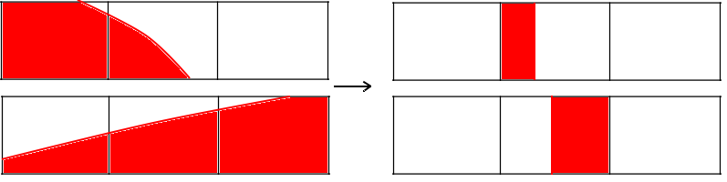
2. Similarly, the Y sweep is performed and each cell is divided into two by line parallel to X.
3.Advection of the interface is then carried out sequentially in both directions. Advection in the X direction is followed by that in Y direction. Advection step includes calculation of the flux across each face of the cell. Consider the case of advection in X direction as shown in the image below.
The middle cell is divided by vertical line and the right part is empty. Now, denote the x component of velocity as u , width of the middle cell as \delta x and time step as \delta t. Since the left face of the cell is already filled, the flux entering through the left face will be u. Till the interface crosses the right face, the flux leaving the right face will be zero. The net flux leaving through right face would be u \delta t - (1-VF)*\delta x. According to the conservation, the change in volume fraction per the unit cell width would be the summation (integral over \delta t) of difference in flux through right and left face.
Piecewise Line Interface Calculation (PLIC)
Here the interface is represented by line with no restriction of being parallel or perpendicular to the sweep direction. The line segment is perpendicular to the gradient of the volume fraction function.
- Approximation of the interface from volume fraction values.
- Advection of the interface according to the known velocity field
Source
- Ubbink, Onno. “Numerical prediction of two fluid systems with sharp interfaces.” (1997).
- Tryggvason, Grétar, Ruben Scardovelli, and Stéphane Zaleski. Direct numerical simulations of gas–liquid multiphase flows. Cambridge University Press, 2011.
- Noh, W.F. and Woodward, P. (1976). SLIC (simple line interface calculation). In Proceedings, Fifth International Conference on Fluid Dynamics (eds. A.I. van de Vooren and P.J. Zandbergen), Lecture Notes in Physics, volume 59. Berlin,Springer, Berlin, pp. 330–340.