Notes from my favorite books1 and 2
Jump to
Material, substantial or total derivative
\begin{equation}
\begin{split}

\frac{D \phi}{D t} &= \frac{\partial \phi}{\partial t} \frac{d t}{d t}+\frac{\partial \phi}{\partial x} \frac{d x}{d t}+\frac{\partial \phi}{\partial y} \frac{d y}{d t}+\frac{\partial \phi}{\partial z} \frac{d z}{d t}\\
&= \frac{\partial \phi}{\partial t} +\frac{\partial \phi}{\partial x} u+\frac{\partial \phi}{\partial y} v+\frac{\partial \phi}{\partial z} w\\
&= \frac{\partial \phi}{\partial t} +\nabla \centerdot \bold{v}\\
\end{split}
\end{equation}
The conservation laws like mass, momentum and energy naturally apply to moving material volumes of fluids, i.e., Lagrangian frame of reference . Hence we need to translate those into Eulerian reference frame, using Reynolds Transport Theorem
Reynolds Transport Theorem
\begin{equation}


\Bigg(\frac{D B}{D t}
\Bigg)_{MV} = \frac{d}{dt} \int_{V} \beta \rho \text{ }dV +\int_{S} \beta \rho v_{r}\cdot n \text{ }dA
\end{equation}
Where, \beta = \frac{dB}{dm}
\bold v_{r} = \begin{cases}
   \bold v   &\text{if CV is fixed}  \\
   \bold v - \bold v_{s}  &\text{if CV is moving with constant velocity, non deforming}  \\
   \bold v(\bold r,t) - \bold v_{s}(t)  &\text{if CV is moving with variable velocity, non deforming }  \\
   \bold v(\bold r,t) - \bold v_{s} (\bold r,t) &\text{if CV is moving with arbitrary velocity and deforming}
\end{cases}
For the fixed control volume, applying Leibniz rule
\begin{equation}
\Bigg(\frac{D B}{D t}
\Bigg)_{MV} =  \int_{V} \frac{\partial}{\partial t}(\beta \rho) \text{ }dV +\int_{S} \beta \rho \bold v_{r}\cdot n \text{ }dA
\end{equation}
Applying the divergence theorem to transform the surface integral into a volume integral, for fixed CV,
\begin{equation}
\Bigg(\frac{D B}{D t}
\Bigg)_{MV} =  \int_{V} \Big[\frac{\partial}{\partial t}(\beta \rho) + \nabla \cdot  \beta \rho \bold v\Big] \text{ }dV
\end{equation}
Conservation of Mass
For conservation of mass, substitute B = m and \beta =1 in (4). Noting that RHS is zero, the integrant has to be zero, which results in
\begin{equation}
\frac{\partial \rho}{\partial t}  + \nabla \cdot  \rho \bold v =0
\end{equation}
Conservation of Linear Momentum
Apply B = \rho \bold v and \beta =\bold v in (4). Noting that RHS becomes force according to Newton’s second law
\begin{equation}
\frac{\partial (\rho \bold v)}{\partial t}  + \nabla \cdot  \rho \bold {vv} =\bold {f_{s}+f_{b}}
\end{equation}
Here \bold {vv} is a diadic product resulting in second order tensor.
Surface forces
Surface force = surface stress x Area.
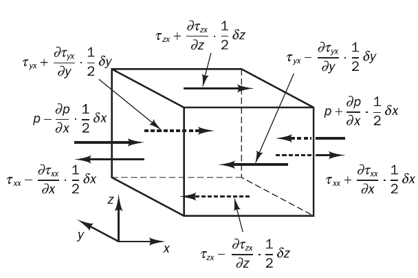
Net force on E and W face is
\Bigg[ \Big( P - \frac{\partial P}{\partial x} \frac{\Delta x}{2} \Big) - \Big( \tau_{xx} - \frac{\partial \tau_{xx}}{\partial x} \frac{\Delta x}{2} \Big) \Bigg]\Delta y \Delta z + \Bigg[ -\Big( P + \frac{\partial P}{\partial x} \frac{\Delta x}{2} \Big) + \Big( \tau_{xx} + \frac{\partial \tau_{xx}}{\partial x} \frac{\Delta x}{2} \Big) \Bigg]\Delta y \Delta zwhich simplifies to:
\Big( - \frac{\partial P}{\partial x} + \frac{\partial \tau_{xx}}{\partial x} \Big) \Delta x \Delta y \Delta z On N and S face:
\frac{\partial \tau_{yx}}{\partial y} \Delta x \Delta y \Delta z On Top and Bottom face:
\frac{\partial \tau_{zx}}{\partial z} \Delta x \Delta y \Delta z Overall force per unit volume in x direction is
\frac{\partial}{\partial x}(-P+ \tau_{xx}) +\frac{\partial \tau_{yx}}{\partial y} +\frac{\partial \tau_{zx}}{\partial z} The x,y and z momentum equations can be written as follows, considering effect of all body forces by one term, S_{Mi}
\rho \frac{Du}{Dt} = \frac{\partial}{\partial x}(-P+ \tau_{xx}) +\frac{\partial \tau_{yx}}{\partial y} +\frac{\partial \tau_{zx}}{\partial z} + S_{Mx}\rho \frac{Dv}{Dt} = \frac{\partial \tau_{xy}}{\partial x}+\frac{\partial}{\partial y}(-P+ \tau_{yy}) +\frac{\partial \tau_{zy}}{\partial z} + S_{My}as conserved variables.
Hence, with surface forces, the momentum equation can be written as:
\begin{equation}
\frac{\partial (\rho \bold v)}{\partial t} + \nabla \cdot \rho \bold {vv} =-\nabla P+ \nabla \cdot \bold \tau +f_{b}
\end{equation}
Navier Stokes Equations
For Newtonian fluids stress tensor\tau is a linear function of strain rate (the anti-symmetric part of velocity gradient just rotate the fluid element)\nabla \bold v , given by
\tau = \mu\Big(\nabla \bold v + (\nabla \bold v )^{T}\Big)+ \lambda(\nabla \cdot \bold v)I\lambda , the second viscosity relate stresses to the volumetric deformation. \lambda = -\frac{2}{3} \mu is a good approximation for gases. For liquids, it is not needed as they are incompressible. Hence,
\begin{equation}
\frac{\partial (\rho \bold v)}{\partial t} + \nabla \cdot \rho \bold {vv} =-\nabla P+ \nabla \cdot \Big[ \mu\Big(\nabla \bold v  + (\nabla \bold v )^{T}\Big)\Big]+ \nabla \Big[\lambda(\nabla \cdot \bold v)\Big] +f_{b}
\end{equation}
for incompressible fluids with constant viscosity:
\begin{equation}
\frac{\partial (\rho \bold v)}{\partial t} + \nabla \cdot \rho \bold {vv} =-\nabla P+   \mu\nabla^{2} \bold v +f_{b}
\end{equation}
Conservation of Energy
Total energy is sum of internal and kinetic energy. Potential energy is accounted in the body force term.
E = m(\hat u+\frac{1}{2}\bold{v\cdot v})From first law of thermodynamics,
\dot E = \dot Q - \dot W = \dot Q_{s} + \dot Q_{b} - \dot W_{s} - \dot W_{b}Work done per unit time is force times velocity
\dot W_{b} = -\int_{v} \bold f_{b} \cdot \bold v \text{ }dV\begin{split}
\dot W_{s} &= -\int_{S} \bold f_{s} \cdot \bold v \text{ }dS\\
&= -\int_{S} (\bold \sigma \cdot n) \cdot \bold v \text{ }dS\\
&= -\int_{V} \nabla \cdot(\bold \sigma \cdot \bold v) \text{ }dV\\
&= -\int_{V} \nabla \cdot(\bold [-PI+\tau]\ \cdot \bold v) \text{ }dV\\
&= -\int_{V} [-\nabla \cdot(P\bold v) +\nabla \cdot (\tau \cdot \bold v) \text{ }]dV\\
\end{split}\dot Q_{b} = \int_{v} \dot q_{b} \text{ }dV\begin{split}
\dot Q_{s} &= -\int_{S} \dot q_{s} \cdot \bold n \text{ }dS\\
&= -\int_{V} \nabla \cdot\dot q_{s} \text{ }dV\\
&= \int_{V} \nabla \cdot K \nabla T \text{ }dV\\
\end{split}Apply Reynolds Transport Theorem with B = \rho e and \beta = e
\int_{V} \Big[\frac{\partial}{\partial t}(\rho e) + \nabla \cdot \rho e \bold v\Big] \text{ }dV = \dot Q_{s} + \dot Q_{b} - \dot W_{s} - \dot W_{b}\begin{equation}
\frac{\partial}{\partial t}(\rho e) + \nabla \cdot \rho e \bold v = \nabla \cdot K \nabla T + \dot q_{b} - \nabla \cdot(P\bold v) + \nabla \cdot (\tau \cdot \bold v) \bold + f_{b} \cdot \bold v
\end{equation}Energy equation is written in multiple forms in terms of specific internal energy, temperature, specific enthalpy and specific total enthalpy. See Moukalled page no 60-65.
Source
- Moukalled F, Mangani L, Darwish M. The finite volume method in computational fluid dynamics. Berlin, Germany:: Springer; 2016.
- Versteeg, H. K., & Malalasekera, W. (2007). An introduction to computational fluid dynamics: The finite volume method. Harlow, England: Pearson Education Ltd.
- Versteeg, H. K., & Malalasekera, W. (2007). An introduction to computational fluid dynamics: The finite volume method. Harlow, England: Pearson Education Ltd.